« Floating exchange rates » : différence entre les versions
Aucun résumé des modifications |
|||
| (7 versions intermédiaires par le même utilisateur non affichées) | |||
| Ligne 2 : | Ligne 2 : | ||
| image = | | image = | ||
| image_caption = | | image_caption = | ||
| cours = [[ | | cours = [[International Economy]] | ||
| faculté = | | faculté = | ||
| département = | | département = | ||
| Ligne 10 : | Ligne 10 : | ||
| enregistrement = | | enregistrement = | ||
| lectures = | | lectures = | ||
* [[ | * [[Ricardo's model: productivity differences as a determinant of trade]] | ||
* [[ | * [[The Heckscher-Ohlin model: differences in factor endowments as a determinant of trade]] | ||
* [[ | * [[Economies of scale as a determinant of trade: beyond comparative advantage]] | ||
* [[ | * [[Trade policy instruments]] | ||
* [[ | * [[Multilateral trade agreements]] | ||
* [[ | * [[Preferential Trade Agreements]] | ||
* [[ | * [[The Free Trade Challenge]] | ||
* [[ | * [[International Macroeconomics: Issues and Overview]] | ||
* [[ | * [[National Accounts and Balance of Payments]] | ||
* [[ | * [[Exchange rates and the foreign exchange market]] | ||
* [[ | * [[Short-term exchange rates: the asset-based approach]] | ||
* [[ | * [[Long-term exchange rates: the monetary approach]] | ||
* [[ | * [[Domestic product and short-term exchange rates]] | ||
* [[ | * [[Floating exchange rates]] | ||
* [[ | * [[Fixed exchange rates and intervention on the foreign exchange market]] | ||
}} | }} | ||
| Ligne 49 : | Ligne 49 : | ||
{{Translations | {{Translations | ||
| fr = Taux de change flottants | | fr = Taux de change flottants | ||
| es = | | es = Tipos de cambio flotantes | ||
}} | }} | ||
| Ligne 107 : | Ligne 107 : | ||
Risk that macroeconomic policy may be recuperated for political purposes (expansive policy just before an election): the anticipation of such behaviour may lead to wage demands and price increases = inflationary bias (self-fulfilling expectations) which led to the independence of many central banks in the 1980s. | Risk that macroeconomic policy may be recuperated for political purposes (expansive policy just before an election): the anticipation of such behaviour may lead to wage demands and price increases = inflationary bias (self-fulfilling expectations) which led to the independence of many central banks in the 1980s. | ||
= | = Model DD-AA: permanent shocks = | ||
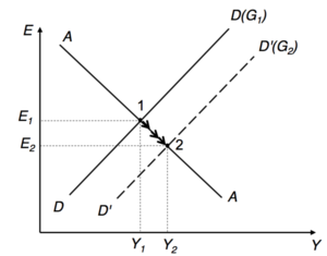
== | == Expansionary fiscal policy == | ||
The change in the expected exchange rate is based on the relationship : <math>E^e = (q)^e(\frac {P}{P^*})</math> | |||
[[File:économie internationale politique modèle DD-AA politique budgétaire expansive 1.png|thumb|center|]] | [[File:économie internationale politique modèle DD-AA politique budgétaire expansive 1.png|thumb|center|]] | ||
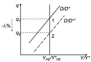
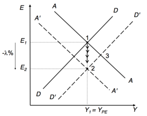
As the level of <math>G</math> has increased, agents anticipate, in the long term, a real appreciation of <math>\lambda</math>% necessary to restore equilibrium in the goods and services market. | |||
Anticipated nominal exchange rate appreciates (same proportion): <math>\hat {E}^e = \hat {q}^e</math> and the rise in domestic demand (due to ↑<math>G</math>) is compensated by a ↓ pf CA. | |||
AA | AA moves downwards by a proportion <math>\lambda</math> vertically to full employment income (<math>Y_1 = Y_{PE}</math> by hypothesis): role of anticipations. | ||
Simultaneous changes => one passes immediately from the point <math>1</math> to the point <math>2</math>. | |||
Nominal appreciation of <math>\lambda</math>% (greater than in the case of a temporary expansion: point <math>3</math> which maintains the economy at its full employment level. | |||
[[File:économie internationale politique modèle DD-AA politique budgétaire expansive 2.png|thumb|center|]] | [[File:économie internationale politique modèle DD-AA politique budgétaire expansive 2.png|thumb|center|]] | ||
No impact on national income (not even in the short term). N.B.: Here <math>\Delta P = 0</math> (<math>\Delta P \neq 0</math> only with monetary shock). | |||
== | == Pexpansive monetary policy == | ||
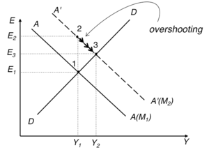
Agents anticipate that, in the long term, an increase in the money supply of <math>\mu</math>% will be reflected in the same proportion on <math>P</math> and on <math>E</math>: role of expectations. | |||
[[File:économie internationale politique modèle DD-AA politique monétaire expansive 1.png|thumb|center|]] | [[File:économie internationale politique modèle DD-AA politique monétaire expansive 1.png|thumb|center|]] | ||
In the short term: | |||
*<math>E^e</math>↑ de <math>\mu</math>%, | *<math>E^e</math>↑ de <math>\mu</math>%, which moves AA upward in the same proportion (vertical to full employment income) -> <math>A'A'</math> (<math>1</math> -> <math>2</math>). | ||
* | *Also, like <math>M</math>↑ => further movement of AA to the right -> <math>A''A''</math> (<math>2</math> -> <math>3</math>). | ||
* | *In <math>3</math> : <math>ED_{BS} > 0</math> -> <math>E</math>↓ => <math>ED_{BS}</math>↓ (<math>3</math> -> <math>4</math>). | ||
=> impact | => impact on <math>Y</math> (↑) even more pronounced than if the shock is temporary (point <math>5</math>). | ||
[[File:économie internationale politique modèle DD-AA politique monétaire expansive 2.png|thumb|center|]] | [[File:économie internationale politique modèle DD-AA politique monétaire expansive 2.png|thumb|center|]] | ||
Gradual price adjustment | |||
As <math>Y > Y_{PE}</math> and <math>M</math> has risen, prices gradually increase until the economy returns to full employment (<math>P_1 \rightarrow P_2</math>) or (<math>4 \rightarrow 2</math>). | |||
= | = DD and AA curves move left until they intersect vertically from <math>Y_1</math> (full employment) to the point <math>2</math> . | ||
=> | => No real long-term consequences (<math>M</math> , <math>E</math> and <math>P</math> all increase in the same proportion): | ||
:::::<math>\hat{M} = \hat{E} = \hat{P} = \mu</math> | :::::<math>\hat{M} = \hat{E} = \hat{P} = \mu</math> | ||
Exchange rate overshooting | |||
== | == Summary: Floating exchange rates == | ||
[[File:économie internationale politique résumé changes flottants 1.png|thumb|center|]] | [[File:économie internationale politique résumé changes flottants 1.png|thumb|center|]] | ||
= | = IS-LM model with floating exchange = | ||
== | == Equilibrium == | ||
[[File:économie internationale IS-LM avec changes flottants équilibre 1.png|thumb|center|]] | [[File:économie internationale IS-LM avec changes flottants équilibre 1.png|thumb|center|]] | ||
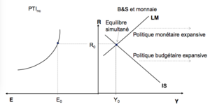
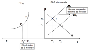
NB | NB: the [[The Keynesian approach and the IS-LM model|IS-LM model]] is a short-term model which is not adapted to capture the long-term effects of an economic policy => in the following we will analyse only the impacts of temporary policies (cf. FT, ch7). | ||
== | == Currency budget shock == | ||
[[File:économie internationale IS-LM avec changes flottants choc monétaire temporaire 1.png|thumb|center|]] | [[File:économie internationale IS-LM avec changes flottants choc monétaire temporaire 1.png|thumb|center|]] | ||
== | == Temporary budget shock == | ||
[[File:économie internationale IS-LM avec changes flottants choc budgétaire temporaire 2.png|thumb|center|]] | [[File:économie internationale IS-LM avec changes flottants choc budgétaire temporaire 2.png|thumb|center|]] | ||
= | = Case Study: The United States Current Account = | ||
== | == US current account 1976-2004 == | ||
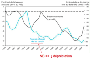
Over the whole period, the real exchange rate and the US current account balance seem to follow a cyclical pattern. | |||
= | = the dollar really appreciates before 1985 and before 2002 (NB: in this graph a rise in the real exchange rate indicates a real appreciation of the dollar), while CA follows the opposite trend. | ||
[[File:économie internationale compte courant des États-Unis compte courant 1976-2004 1.png|thumb|center|]] | [[File:économie internationale compte courant des États-Unis compte courant 1976-2004 1.png|thumb|center|]] | ||
Can the DD-AA model (KO, ch.17) explain these developments? | |||
== | == Explanation == | ||
DD-AA model and expansive fiscal policy: as just seen above, under the DD-AA model an expansive fiscal policy leads to a real appreciation of the national currency and a current account deficit. This works well with the early 1980s and early 2000s: the two governments involved (Reagan or Bush junior) both reduced taxes and increased military spending. | |||
What causes the pendulum to swing back? | |||
Suggested KO: wealth effect (not formally incorporated in the DD-AA model) = as the current account deficit widens, the wealth of residents falls relative to that of non-residents (see chapter 10). Since there is a national preference, this should lead to a decline in the relative demand for domestic products, and thus to a real depreciation of the national currency. If the latter is correctly anticipated by agents, this immediately generates a depreciation of the national currency, which gradually corrects the current account deficit. | |||
== Puzzles == | == Puzzles == | ||
1. | 1. As soon as it noticed a fall in industrial production following the crisis caused by the 2000-2001 financial bubble (new technologies), the FED lowered interest rates to mitigate the effects of the recession = expansive monetary policy, which should have led, according to our DD-AA approach, to a depreciation of the dollar. However, the USD continued to appreciate until 2002. Why did it do so? | ||
Possible explanation: anticipation of future appreciation of the US currency based on two elements: | |||
#Bush, | #Bush, narrowly elected, announces tax cuts = expansive fiscal policy. | ||
# | #The 9/11 attacks would certainly call for an expansive fiscal policy. | ||
2. | 2. From 2002 onwards the US dollar started to depreciate considerably. In spite of this, the trade balance continues to remain heavily in deficit and there is no evidence of improvement. Why? | ||
Possible explanation: US domestic consumption too high and savings too low in relation to investments → strong international imbalances (see end of chapter 10). | |||
Conclusion : | Conclusion: One must remain cautious in the analysis. There are enough exogenous variables in the model to make it consistent with virtually all macroeconomic developments! | ||
= Annexes = | = Annexes = | ||
Version actuelle datée du 23 avril 2020 à 15:05
| Professeur(s) | |
|---|---|
| Cours | International Economy |
Lectures
- Ricardo's model: productivity differences as a determinant of trade
- The Heckscher-Ohlin model: differences in factor endowments as a determinant of trade
- Economies of scale as a determinant of trade: beyond comparative advantage
- Trade policy instruments
- Multilateral trade agreements
- Preferential Trade Agreements
- The Free Trade Challenge
- International Macroeconomics: Issues and Overview
- National Accounts and Balance of Payments
- Exchange rates and the foreign exchange market
- Short-term exchange rates: the asset-based approach
- Long-term exchange rates: the monetary approach
- Domestic product and short-term exchange rates
- Floating exchange rates
- Fixed exchange rates and intervention on the foreign exchange market
What is the impact of macroeconomic policies (↑ or ↑) under a floating exchange rate regime?
Does a temporary shock () have the same effect on the exchange rate as a permanent shock ()?
Can the evolution of the US current account be explained on the basis of the full model (DD-AA)?
Application of the DD-AA model to analyse the effects of fiscal and monetary policies.
Two possible situations :
- Floating exchange rates (this chapter)
- Fixed exchange rates (next chapter)
We start from a long-term situation where , .
We consider an expansionary shock (↑ of or ). Distinction between:
Temporary shock doesn't change currency expectations (\Delta E^e = 0</math>).
Permanent shock modifies exchange rate expectations (); in this case we also distinguish short-term effects () from long-term effects ().
Floating exchange rates[modifier | modifier le wikicode]
Most developed countries adopt a floating exchange rate regime = the government does not systematically intervene to try to maintain a parity against a base currency → continuous fluctuations.
Case Swiss franc (CHF) - euro (EUR)

Model DD-AA: Temporary shocks[modifier | modifier le wikicode]
Politique budgétaire expansive[modifier | modifier le wikicode]
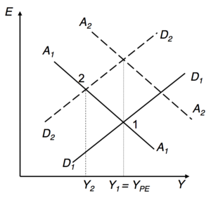
Temporary shocks =>
↗ => DD to the right => given, ED of goods and services => ↗ =>Currency ED => ↗ => ED of national currency => ↘ (ds movement along AA). This until equilibrium is restored in all markets at the point (but with a CA↘ through an appreciation of the national currency).
Expansionary monetary policy[modifier | modifier le wikicode]
Chocs temporaires =>
↗ => AA to the right => to , -> ↘ => -> ↗ = feedback on A’A’ (immediate adaptation), but with CA higher than initially => => ↗ => gradual transition from the point to the point (= partial compensation for the initial depreciation of the national currency).
Finally, at the point the AC improved through the depreciation of the national currency.
Policy of maintaining full employment[modifier | modifier le wikicode]
Initially
Temporary negative shock : ⟶ => 1 ⟶ 2 et
How to restore ? Either by:
- Monetary expansion ( ⟶ )
- Fiscal expansion ( ⟶ )
Or: combining monetary and fiscal policy
NB1: Even if the effect of these two interventions on output is identical, monetary policy and fiscal policy are not equivalent in their impact on the exchange rate.
NB2: What interventions can be imagined to counteract the recessionary effect of a temporary increase in the demand for money?
Remarks on stabilization policies[modifier | modifier le wikicode]
The short-term impact of macroeconomic policies may not occur at the desired time (the problem of timing, which affects fiscal policy more strongly).
Increasing government deficit as a result of an expansive fiscal policy weighs on future generations.
Risk that macroeconomic policy may be recuperated for political purposes (expansive policy just before an election): the anticipation of such behaviour may lead to wage demands and price increases = inflationary bias (self-fulfilling expectations) which led to the independence of many central banks in the 1980s.
Model DD-AA: permanent shocks[modifier | modifier le wikicode]
Expansionary fiscal policy[modifier | modifier le wikicode]
The change in the expected exchange rate is based on the relationship :
As the level of has increased, agents anticipate, in the long term, a real appreciation of % necessary to restore equilibrium in the goods and services market.
Anticipated nominal exchange rate appreciates (same proportion): and the rise in domestic demand (due to ↑) is compensated by a ↓ pf CA.
AA moves downwards by a proportion vertically to full employment income ( by hypothesis): role of anticipations.
Simultaneous changes => one passes immediately from the point to the point .
Nominal appreciation of % (greater than in the case of a temporary expansion: point which maintains the economy at its full employment level.
No impact on national income (not even in the short term). N.B.: Here ( only with monetary shock).
Pexpansive monetary policy[modifier | modifier le wikicode]
Agents anticipate that, in the long term, an increase in the money supply of % will be reflected in the same proportion on and on : role of expectations.
In the short term:
- ↑ de %, which moves AA upward in the same proportion (vertical to full employment income) -> ( -> ).
- Also, like ↑ => further movement of AA to the right -> ( -> ).
- In : -> ↓ => Échec de l’analyse (MathML avec SVG ou PNG en secours (recommandé pour les navigateurs modernes et les outils d’accessibilité) : réponse non valide(« Math extension cannot connect to Restbase. ») du serveur « https://en.wikipedia.org/api/rest_v1/ » :): {\displaystyle ED_{BS}} ↓ ( -> Échec de l’analyse (MathML avec SVG ou PNG en secours (recommandé pour les navigateurs modernes et les outils d’accessibilité) : réponse non valide(« Math extension cannot connect to Restbase. ») du serveur « https://en.wikipedia.org/api/rest_v1/ » :): {\displaystyle 4} ).
=> impact on Échec de l’analyse (MathML avec SVG ou PNG en secours (recommandé pour les navigateurs modernes et les outils d’accessibilité) : réponse non valide(« Math extension cannot connect to Restbase. ») du serveur « https://en.wikipedia.org/api/rest_v1/ » :): {\displaystyle Y} (↑) even more pronounced than if the shock is temporary (point Échec de l’analyse (MathML avec SVG ou PNG en secours (recommandé pour les navigateurs modernes et les outils d’accessibilité) : réponse non valide(« Math extension cannot connect to Restbase. ») du serveur « https://en.wikipedia.org/api/rest_v1/ » :): {\displaystyle 5} ).
Gradual price adjustment
As Échec de l’analyse (MathML avec SVG ou PNG en secours (recommandé pour les navigateurs modernes et les outils d’accessibilité) : réponse non valide(« Math extension cannot connect to Restbase. ») du serveur « https://en.wikipedia.org/api/rest_v1/ » :): {\displaystyle Y > Y_{PE}} and Échec de l’analyse (MathML avec SVG ou PNG en secours (recommandé pour les navigateurs modernes et les outils d’accessibilité) : réponse non valide(« Math extension cannot connect to Restbase. ») du serveur « https://en.wikipedia.org/api/rest_v1/ » :): {\displaystyle M} has risen, prices gradually increase until the economy returns to full employment (Échec de l’analyse (MathML avec SVG ou PNG en secours (recommandé pour les navigateurs modernes et les outils d’accessibilité) : réponse non valide(« Math extension cannot connect to Restbase. ») du serveur « https://en.wikipedia.org/api/rest_v1/ » :): {\displaystyle P_1 \rightarrow P_2} ) or (Échec de l’analyse (MathML avec SVG ou PNG en secours (recommandé pour les navigateurs modernes et les outils d’accessibilité) : réponse non valide(« Math extension cannot connect to Restbase. ») du serveur « https://en.wikipedia.org/api/rest_v1/ » :): {\displaystyle 4 \rightarrow 2} ).
= DD and AA curves move left until they intersect vertically from Échec de l’analyse (MathML avec SVG ou PNG en secours (recommandé pour les navigateurs modernes et les outils d’accessibilité) : réponse non valide(« Math extension cannot connect to Restbase. ») du serveur « https://en.wikipedia.org/api/rest_v1/ » :): {\displaystyle Y_1} (full employment) to the point Échec de l’analyse (MathML avec SVG ou PNG en secours (recommandé pour les navigateurs modernes et les outils d’accessibilité) : réponse non valide(« Math extension cannot connect to Restbase. ») du serveur « https://en.wikipedia.org/api/rest_v1/ » :): {\displaystyle 2} .
=> No real long-term consequences (Échec de l’analyse (MathML avec SVG ou PNG en secours (recommandé pour les navigateurs modernes et les outils d’accessibilité) : réponse non valide(« Math extension cannot connect to Restbase. ») du serveur « https://en.wikipedia.org/api/rest_v1/ » :): {\displaystyle M} , Échec de l’analyse (MathML avec SVG ou PNG en secours (recommandé pour les navigateurs modernes et les outils d’accessibilité) : réponse non valide(« Math extension cannot connect to Restbase. ») du serveur « https://en.wikipedia.org/api/rest_v1/ » :): {\displaystyle E} and Échec de l’analyse (MathML avec SVG ou PNG en secours (recommandé pour les navigateurs modernes et les outils d’accessibilité) : réponse non valide(« Math extension cannot connect to Restbase. ») du serveur « https://en.wikipedia.org/api/rest_v1/ » :): {\displaystyle P} all increase in the same proportion):
- Échec de l’analyse (MathML avec SVG ou PNG en secours (recommandé pour les navigateurs modernes et les outils d’accessibilité) : réponse non valide(« Math extension cannot connect to Restbase. ») du serveur « https://en.wikipedia.org/api/rest_v1/ » :): {\displaystyle \hat{M} = \hat{E} = \hat{P} = \mu}
Exchange rate overshooting
Summary: Floating exchange rates[modifier | modifier le wikicode]
IS-LM model with floating exchange[modifier | modifier le wikicode]
Equilibrium[modifier | modifier le wikicode]
NB: the IS-LM model is a short-term model which is not adapted to capture the long-term effects of an economic policy => in the following we will analyse only the impacts of temporary policies (cf. FT, ch7).
Currency budget shock[modifier | modifier le wikicode]
Temporary budget shock[modifier | modifier le wikicode]
Case Study: The United States Current Account[modifier | modifier le wikicode]
US current account 1976-2004[modifier | modifier le wikicode]
Over the whole period, the real exchange rate and the US current account balance seem to follow a cyclical pattern. = the dollar really appreciates before 1985 and before 2002 (NB: in this graph a rise in the real exchange rate indicates a real appreciation of the dollar), while CA follows the opposite trend.
Can the DD-AA model (KO, ch.17) explain these developments?
Explanation[modifier | modifier le wikicode]
DD-AA model and expansive fiscal policy: as just seen above, under the DD-AA model an expansive fiscal policy leads to a real appreciation of the national currency and a current account deficit. This works well with the early 1980s and early 2000s: the two governments involved (Reagan or Bush junior) both reduced taxes and increased military spending.
What causes the pendulum to swing back?
Suggested KO: wealth effect (not formally incorporated in the DD-AA model) = as the current account deficit widens, the wealth of residents falls relative to that of non-residents (see chapter 10). Since there is a national preference, this should lead to a decline in the relative demand for domestic products, and thus to a real depreciation of the national currency. If the latter is correctly anticipated by agents, this immediately generates a depreciation of the national currency, which gradually corrects the current account deficit.
Puzzles[modifier | modifier le wikicode]
1. As soon as it noticed a fall in industrial production following the crisis caused by the 2000-2001 financial bubble (new technologies), the FED lowered interest rates to mitigate the effects of the recession = expansive monetary policy, which should have led, according to our DD-AA approach, to a depreciation of the dollar. However, the USD continued to appreciate until 2002. Why did it do so? Possible explanation: anticipation of future appreciation of the US currency based on two elements:
- Bush, narrowly elected, announces tax cuts = expansive fiscal policy.
- The 9/11 attacks would certainly call for an expansive fiscal policy.
2. From 2002 onwards the US dollar started to depreciate considerably. In spite of this, the trade balance continues to remain heavily in deficit and there is no evidence of improvement. Why?
Possible explanation: US domestic consumption too high and savings too low in relation to investments → strong international imbalances (see end of chapter 10).
Conclusion: One must remain cautious in the analysis. There are enough exogenous variables in the model to make it consistent with virtually all macroeconomic developments!
Annexes[modifier | modifier le wikicode]
References[modifier | modifier le wikicode]
- ↑ Page personnelle de Federica Sbergami sur le site de l'Université de Genève
- ↑ Page personnelle de Federica Sbergami sur le site de l'Université de Neuchâtel
- ↑ Page personnelle de Federica Sbergami sur Research Gate
- ↑ Céline Carrère - Faculté d'économie et de management - UNIGE
- ↑ Céline Carrère - Google Scholar Citations
- ↑ Director Céline Carrère - Rectorat - UNIGE
- ↑ Céline Carrère | Sciences Po - Le Laboratoire Interdisciplinaire d'Evaluation des Politiques Publiques (LIEPP)
- ↑ Céline Carrere - EconPapers
- ↑ Céline Carrère's research works - ResearchGate
- ↑ http://fx.sauder.ubc.ca/data.html


