« Aggregate demand and supply » : différence entre les versions
Aucun résumé des modifications |
|||
| (8 versions intermédiaires par le même utilisateur non affichées) | |||
| Ligne 2 : | Ligne 2 : | ||
| image = | | image = | ||
| image_caption = | | image_caption = | ||
| cours = [[Introduction | | cours = [[Introduction to Macroeconomics]] | ||
| faculté = | | faculté = | ||
| département = | | département = | ||
| professeurs = | | professeurs = | ||
*[[Federica Sbergami|Sbergami, Federica]]<ref>[https://www.unige.ch/gsem/en/research/faculty/all/federica-sbergami/ Page personnelle de Federica Sbergami sur le site de l'Université de Genève]</ref><ref>[https://www.unine.ch/irene/home/equipe/federica_sbergami.html Page personnelle de Federica Sbergami sur le site de l'Université de Neuchâtel]</ref><ref>[https://www.researchgate.net/scientific-contributions/14836393_Federica_Sbergami Page personnelle de Federica Sbergami sur Research Gate]</ref> | *[[Federica Sbergami|Sbergami, Federica]]<ref>[https://www.unige.ch/gsem/en/research/faculty/all/federica-sbergami/ Page personnelle de Federica Sbergami sur le site de l'Université de Genève]</ref><ref>[https://www.unine.ch/irene/home/equipe/federica_sbergami.html Page personnelle de Federica Sbergami sur le site de l'Université de Neuchâtel]</ref><ref>[https://www.researchgate.net/scientific-contributions/14836393_Federica_Sbergami Page personnelle de Federica Sbergami sur Research Gate]</ref> | ||
*[[Nicolas Maystre]]<ref>Researchgate.net - [https://www.researchgate.net/profile/Nicolas_Maystre Nicolas Maystre]</ref><ref>Google Scholar - [https://scholar.google.com/citations?user=B73U0wsAAAAJ&hl=en Nicolas Maystre]</ref><ref>VOX, CEPR Policy Portal - [https://voxeu.org/users/nicolasmaystre0 Nicolas Maystre]</ref><ref>[http://nicolas.maystre.ch/ Nicolas Maystre's webpage]</ref><ref>Cairn.ingo - [https://www.cairn.info/publications-de-Nicolas-Maystre--104530.htm Nicolas Maystre]</ref><ref>Linkedin - [https://www.linkedin.com/in/nicolas-maystre-82660737/?originalSubdomain=ch Nicolas Maystre]</ref><ref>Academia.edu - | *[[Nicolas Maystre]]<ref>Researchgate.net - [https://www.researchgate.net/profile/Nicolas_Maystre Nicolas Maystre]</ref><ref>Google Scholar - [https://scholar.google.com/citations?user=B73U0wsAAAAJ&hl=en Nicolas Maystre]</ref><ref>VOX, CEPR Policy Portal - [https://voxeu.org/users/nicolasmaystre0 Nicolas Maystre]</ref><ref>[http://nicolas.maystre.ch/ Nicolas Maystre's webpage]</ref><ref>Cairn.ingo - [https://www.cairn.info/publications-de-Nicolas-Maystre--104530.htm Nicolas Maystre]</ref><ref>Linkedin - [https://www.linkedin.com/in/nicolas-maystre-82660737/?originalSubdomain=ch Nicolas Maystre]</ref><ref>Academia.edu - [https://unctad.academia.edu/NicolasMaystre Nicolas Maystre]</ref> | ||
| enregistrement = | | enregistrement = | ||
| lectures = | | lectures = | ||
*[[ | *[[Introductory aspects of macroeconomics]] | ||
*[[ | *[[Gross Domestic Product (GDP)]] | ||
*[[ | *[[Consumer Price Index (CPI)]] | ||
*[[Production | *[[Production and economic growth]] | ||
*[[ | *[[Unemployment]] | ||
*[[ | *[[Financial Market]] | ||
*[[ | *[[The monetary system]] | ||
*[[ | *[[Monetary growth and inflation]] | ||
*[[ | *[[Open Macroeconomics: Basic Concepts]] | ||
*[[ | *[[Open Macroeconomics: the Exchange Rate]] | ||
*[[ | *[[Equilibrium in an open economy]] | ||
*[[ | *[[The Keynesian approach and the IS-LM model]] | ||
*[[ | *[[Aggregate demand and supply]] | ||
*[[ | *[[The impact of monetary and fiscal policies]] | ||
*[[Trade-off | *[[Trade-off between inflation and unemployment]] | ||
*[[ | *[[Response to the 2008 Financial Crisis and International Cooperation]] | ||
}} | }} | ||
As we saw in the previous chapter, economies fluctuate widely around their level of full employment output. During a recession there will be a decline in economic activity and an underutilization of production factors (including unemployment). During a boom or expansion there will be an over-utilization of production factors. | |||
<gallery mode="packed-hover" widths="200px" heights="200px"> | <gallery mode="packed-hover" widths="200px" heights="200px"> | ||
| Ligne 41 : | Ligne 41 : | ||
{{Translations | {{Translations | ||
| fr = Demande et offre agrégée | | fr = Demande et offre agrégée | ||
| es = | | es = Demanda y oferta agregadas | ||
}} | }} | ||
| Ligne 79 : | Ligne 79 : | ||
[[Fichier:Intromacro Forme et position de la DA 1.png|400px|vignette|centré]] | [[Fichier:Intromacro Forme et position de la DA 1.png|400px|vignette|centré]] | ||
= | =Short- and long-term offer= | ||
== | ==Short- and long-term aggregate offer== | ||
In the long run the aggregate offer curve (AO) is totally inelastic, because the quantity produced of goods and services at full employment does not depend on prices, but on the available quantities of the factors of production and technical knowledge → The aggregate supply that corresponds to the level of full employment (or natural, or potential) production is therefore not dependent on prices and shifts when the supply of one of the factors of production changes, or when there is a change in technological knowledge. | |||
In the short run the aggregate offer curve (AO) is elastic, and the quantity of goods and services on offer increases or decreases with the price level in the economy. Because of frictions in the economic system in the short run, which cause the price level expected by individuals to be different from the observed price level (market imperfections), when the observed price level is higher (lower) than the expected price level, one will produce more (less) than at the level of full employment. | |||
== | ==AO and the general price level== | ||
# | #Sticky wages theory: when prices fall, wages take longer to adjust (contracts are fixed for relatively long periods). Producers therefore face lower prices, but with costs as high as they were before the price drop → they will reduce the level of production and employment → AO falls. | ||
# | #Sticky prices theory: prices fall, but some companies take a long time to adjust them (menu costs). Demand is falling for those firms that do not adjust prices quickly, so they will have to reduce the quantities produced and employment → AO is falling. | ||
# | #Misperception theory: prices are falling, but some firms do not realize that this is a general decline and think that it is only their prices that are falling (relative price decline), and therefore reduce their output and employment → AO is falling. | ||
Whenever there is a gap between the observed price and the expected price, this gap is reflected to a greater or lesser extent (depending on an alpha parameter) in a change in supply relative to the level of full employment output. | |||
:: | ::Short-term output (Y) = Full employment output (<math>Y_PE</math>) + α [Observed price (P) - Anticipated price (<math>P^e</math>)]]. | ||
FO is a direct function of prices. | |||
== | ==Shifts in the short-term offer curve== | ||
Shocks that can influence the AO's position: | |||
In the short term <math>Y = Y_PE + \alpha (P - P^e)</math> => the short term supply function shifts for the same reasons that cause a shift in the long term supply curve: increased productivity or supply of production factors (<math>L</math>, <math>K</math>, <math>H</math>, or <math>N</math>) or improved technological knowledge (<math>A</math>). | |||
But there is an additional reason that causes the short-term OA curve to shift: changes in price expectations cause shifts in aggregate short-term supply. In particular, a rise in the expected price causes a short-term OA ↓ for any observed price (moving the curve to the left → it is anticipated that production costs will rise and the level of production at observed price parity is lowered). | |||
== | ==Shape and movement of the AO== | ||
[[Fichier:Intromacro Forme et déplacement de OA 1.png|400px|vignette|centré]] | [[Fichier:Intromacro Forme et déplacement de OA 1.png|400px|vignette|centré]] | ||
| Ligne 113 : | Ligne 113 : | ||
[[Fichier:Intromacro Forme et déplacement de OA 2.png|400px|vignette|centré]] | [[Fichier:Intromacro Forme et déplacement de OA 2.png|400px|vignette|centré]] | ||
= | =Short-term fluctuations= | ||
== | ==Equilibrium== | ||
[[Fichier:Intromacro daod équilibre 1.png|400px|vignette|centré]] | [[Fichier:Intromacro daod équilibre 1.png|400px|vignette|centré]] | ||
== | ==Moving the Aggregate Demand AD== | ||
A contraction of the AD (generalized pessimism, decrease of <math>G</math>, ...) causes : | |||
1. | 1. in the short term, a decrease in production, and a drop in prices (recession) ... | ||
[[Fichier:Intromacro Déplacement de la DA 1.png|400px|vignette|centré]] | [[Fichier:Intromacro Déplacement de la DA 1.png|400px|vignette|centré]] | ||
A contraction of the AD (generalized pessimism, decrease of <math>G</math>, ...) causes : | |||
... 2. | ... 2. in the long term, a decrease in prices but no decrease in output (because expectations adjust, which shifts the aggregate supply to the right: in <math>B</math>, <math>Y < Y_PE</math> → expectations of a gradual decrease in prices → nominal wages adjust → production costs ↓ → supply ↑ → we come back to <math>Y_PE</math>) | ||
[[Fichier:Intromacro Déplacement de la DA 2.png|400px|vignette|centré]] | [[Fichier:Intromacro Déplacement de la DA 2.png|400px|vignette|centré]] | ||
NB: | NB: in the short term, fluctuations! Y</math>Y</math> is temporarily below <math>Y_PE</math>. In the long term the demand shock is completely absorbed by a price change and <math>Y</math> <revenues to <math>Y_PE</math>. | ||
== | ==Displacement of the AO== | ||
A contraction of the AO (natural disaster, wage demands, ...) causes : | |||
1. | 1. in the short term "stagflation": P↑ and Y↓ = recession + inflation ... | ||
[[Fichier:Intromacro Déplacement de l’OA 1.png|400px|center|vignette|gauche]] | [[Fichier:Intromacro Déplacement de l’OA 1.png|400px|center|vignette|gauche]] | ||
A contraction of the AO (natural disaster, wage demands, ...) causes : | |||
... 2. | ... 2. in the long term, nothing because the adjustment of expectations will cause a shift in the aggregate supply curve to its initial position (same reasoning as for the long-term effects of a fall in AD: <math>Y < Y_PE</math> → expectations of a gradual fall in prices → ...) | ||
[[Fichier:Intromacro Déplacement de l’OA 2.png|400px|center|vignette|gauche|Les fluctuations de l'output de court terme sont corrigées automatiquement dans le long terme.]] | [[Fichier:Intromacro Déplacement de l’OA 2.png|400px|center|vignette|gauche|Les fluctuations de l'output de court terme sont corrigées automatiquement dans le long terme.]] | ||
3. | 3. In the case of a government intervention aimed at counteracting the initial decline in AO there is a risk of further damage (↑P). This is one of the reasons why, according to the monetarists, the government should not intervene in the economic system (risk of introducing even more serious distortions). | ||
[[Fichier:Intromacro Déplacement de l’OA 3.png|400px|center|vignette|gauche|NB.: Une augmentation de la DA (intervention du gouvernement ayant comme but de s’opposer à la contraction initiale de l’OA) provoque encore plus d’inflation.]] | [[Fichier:Intromacro Déplacement de l’OA 3.png|400px|center|vignette|gauche|NB.: Une augmentation de la DA (intervention du gouvernement ayant comme but de s’opposer à la contraction initiale de l’OA) provoque encore plus d’inflation.]] | ||
== | ==Which model for the interest rate?== | ||
In Chapter 6 we determined the interest rate as the equilibrium rate that equals the amount of loanable funds offered by savers and the amount of loanable funds demanded to finance the investment. In Chapter 11 we determined the interest rate as the equilibrium rate that equals the demand for and supply of money. Now that we have clarified the short- and long-term concepts, it is easy to show that the lendable funds model and the liquidity preference model are compatible and consistent. | |||
In the short run, a fall in the interest rate caused by a ↑ of M increases investment and thus GDP. The ↑ of GDP in turn increases consumption, but also savings (see graphs on the next page). By how much does saving increase? Exactly by the increase in I (at equilibrium: I = S). | |||
[[Fichier:Intromacro quel modèle pour le taux d interet court terme 1.png|400px|vignette|centré| | [[Fichier:Intromacro quel modèle pour le taux d interet court terme 1.png|400px|vignette|centré|In the short term it is the supply and demand for money that determines the interest rate and the market for loanable funds adjusts.]] | ||
In the long run, we know that the supply of money does not influence the interest rate and that any change in M translates into a proportional change in P. As the general price level ↑ increases, the demand for money increases in the same proportion (shift in the curve). With the price adjustment, Y returns to its full employment level (and thus the supply function of lendable funds to its initial position) and the interest rate to its initial level (see charts on the next page). | |||
[[Fichier:Intromacro quel modèle pour le taux d interet long terme 1.png|400px|vignette|centré|In the long term, it is the supply and demand for loanable funds from the product of full employment that determines the interest rate.]] | |||
==Short vs. long term== | |||
Reminder of the main differences between long-term and short-term approaches in macroeconomics. | |||
Three central macroeconomic variables to understand this distinction : | |||
*the production of goods and services; | |||
*the real interest rate; | |||
*the general price level. | |||
==In the long term== | |||
#Production is determined by the supply of capital and labour and the production technology available to transform these factors into a certain level of output (which is often referred to as the "natural" rate of production). | |||
#For any level of output, the real interest rate balances the supply and demand for loanable funds. | |||
#The general price level then balances the supply and demand for money. Changes in the supply of money lead to proportional changes in the general price level. | |||
N.B. The three propositions above represent the essence of classical economic theory. The majority of economists believe that these propositions are adequate to describe the functioning of the economy in the long run. | |||
==In the short term== | |||
The proposals in the previous point are no longer valid. Thus, in the short term, it is preferable to think of the functioning of the economy as follows: | |||
#The general price level is fixed at a certain value (determined according to past expectations) and in the short term it reacts only weakly to changes in economic conditions. | |||
#For any general price level,the interest rate adjusts to balance the supply and demand for money. | |||
#The level of output responds to changes in the aggregate demand for goods and services, which is determined in part by the interest rate that achieves equilibrium in the money market. | |||
=Summary= | |||
Economic fluctuations are difficult to predict and economists use the Aggregate Demand (AD) and Aggregate Offer (AO) model to analyze these fluctuations in the short term. | |||
Aggregate demand has a negative slope in space (quantity, general price level) due to a "wealth" effect, an effect on the interest rate and an effect on the trade balance. | |||
Any shock that affects consumption, investment, government spending and the trade balance will cause movements in the demand function. | |||
In the long term, aggregate supply is vertical, but in the short term it has a positive slope, in space (quantity, general price level), in time (quantity, general price level) and in space (quantity, general price level). | |||
There are 3 possible explanations for this positive short-term slope: rigid wages, rigid prices, or misperceptions. | |||
Shifts in the short-term supply curve are explained by the same factors as shifts in the long-term supply curve. | |||
But there is an additional reason: changes in expectations about the price level will affect the position of the supply curve. | |||
Changes in demand and aggregate supply will cause short-term changes in output and price levels. | |||
But in the long run changes in aggregate demand will only cause changes in the price level and the aggregate supply will readjust and return to the initial equilibrium. | |||
In the short term one can try to correct the impact of a contraction in aggregate supply by stimulating the DA (with an increase in public expenditure for example), and this will increase output in the short term, but will also cause an increase in the general price level greater than that initially caused by the contraction of the AO. | |||
=Annexes= | =Annexes= | ||
Version actuelle datée du 4 avril 2020 à 15:04
| Professeur(s) | |
|---|---|
| Cours | Introduction to Macroeconomics |
Lectures
- Introductory aspects of macroeconomics
- Gross Domestic Product (GDP)
- Consumer Price Index (CPI)
- Production and economic growth
- Unemployment
- Financial Market
- The monetary system
- Monetary growth and inflation
- Open Macroeconomics: Basic Concepts
- Open Macroeconomics: the Exchange Rate
- Equilibrium in an open economy
- The Keynesian approach and the IS-LM model
- Aggregate demand and supply
- The impact of monetary and fiscal policies
- Trade-off between inflation and unemployment
- Response to the 2008 Financial Crisis and International Cooperation
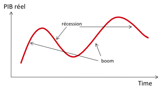
As we saw in the previous chapter, economies fluctuate widely around their level of full employment output. During a recession there will be a decline in economic activity and an underutilization of production factors (including unemployment). During a boom or expansion there will be an over-utilization of production factors.

Taux de chômage en Suisse (1990 - 2008)


Economists use the aggregated demand and supply model (DA-OA) to analyse fluctuations in economic activity around the long-term trend.
The DA-OA and IS-LM models are closely related. In particular, it can easily be shown that the aggregate demand function captures all the pairs (Y, P) that ensure the simultaneous equilibrium of the B&S market (IS curve) and the money market (LM curve). The main difference between these two models is that the IS-LM model considers the general price level as exogenous and is therefore not equipped to analyse the long-term effects of macroeconomic policies. In contrast, the DA-OA model is able to show how the general price level and real GDP are determined simultaneously.
Aggregate demand[modifier | modifier le wikicode]
Aggregate demand[modifier | modifier le wikicode]
Aggregate demand (AD) indicates the quantity of goods and services produced in the domestic economy that is demanded by consumers, investors, government and the rest of the world for each general price level in the economy (NB.: Total expenditure E in the IS-LM model rather highlights the link between demand and income):

Aggregate demand, like demand for a good, decreases with the price level => DA(P) , but for reasons that are different from those - specific to the microeconomy.
One of the reasons why demand for a good increases when the price decreases is the substitution effect with other goods. If the price of coffee decreases relative to the price of chocolate (relative price change), more coffee is consumed relative to chocolate (assuming that coffee and chocolate are substitutable goods).
With aggregate demand, there is no substitution effect by definition.
AD and the general price level[modifier | modifier le wikicode]
- Wealth effect and consumption: as we saw in chapter 8, when prices fall individuals feel richer, because a 1$ can buy more than before (the value of money ↑) → their consumption increases → AD increases.
- The effect on interest rate and investment: as we saw in chapter 8, when prices ↓ households need less money for transaction reasons → they offer more loanable funds at r parity → this causes a decrease in the equilibrium interest rate and thus an increase in investment because it becomes cheaper to borrow to invest (more investments become profitable with a lower interest rate) → AD increases.
- The effect on the trade balance: if the prices of locally produced goods fall, the demand for these goods increases in relation to the demand for goods produced in the WDR → exports increase and imports decrease → AD increases.
The AD is an inverse function of prices.
Travel of the AD[modifier | modifier le wikicode]
Price is not the only factor influencing aggregate demand → exogenous shocks that can influence the position of the DA :
- Change in willingness to consume (versus save) = marginal propensity to consume (mpc). This can be caused in turn by an increase in life expectancy, by expectations of a recession or boom, by a property bubble, by an exogenous variation in household wealth, etc.
- Change in willingness to invest (expectations over the business cycle)
- Changes in government spending
- Changes in net demand from the rest of the world: a recession abroad will reduce domestic net exports and thus cause a shift in AD.
Form and position of the AD[modifier | modifier le wikicode]

Short- and long-term offer[modifier | modifier le wikicode]
Short- and long-term aggregate offer[modifier | modifier le wikicode]
In the long run the aggregate offer curve (AO) is totally inelastic, because the quantity produced of goods and services at full employment does not depend on prices, but on the available quantities of the factors of production and technical knowledge → The aggregate supply that corresponds to the level of full employment (or natural, or potential) production is therefore not dependent on prices and shifts when the supply of one of the factors of production changes, or when there is a change in technological knowledge.
In the short run the aggregate offer curve (AO) is elastic, and the quantity of goods and services on offer increases or decreases with the price level in the economy. Because of frictions in the economic system in the short run, which cause the price level expected by individuals to be different from the observed price level (market imperfections), when the observed price level is higher (lower) than the expected price level, one will produce more (less) than at the level of full employment.
AO and the general price level[modifier | modifier le wikicode]
- Sticky wages theory: when prices fall, wages take longer to adjust (contracts are fixed for relatively long periods). Producers therefore face lower prices, but with costs as high as they were before the price drop → they will reduce the level of production and employment → AO falls.
- Sticky prices theory: prices fall, but some companies take a long time to adjust them (menu costs). Demand is falling for those firms that do not adjust prices quickly, so they will have to reduce the quantities produced and employment → AO is falling.
- Misperception theory: prices are falling, but some firms do not realize that this is a general decline and think that it is only their prices that are falling (relative price decline), and therefore reduce their output and employment → AO is falling.
Whenever there is a gap between the observed price and the expected price, this gap is reflected to a greater or lesser extent (depending on an alpha parameter) in a change in supply relative to the level of full employment output.
- Short-term output (Y) = Full employment output () + α [Observed price (P) - Anticipated price ()]].


FO is a direct function of prices.
Shifts in the short-term offer curve[modifier | modifier le wikicode]
Shocks that can influence the AO's position:
In the short term => the short term supply function shifts for the same reasons that cause a shift in the long term supply curve: increased productivity or supply of production factors (, , , or ) or improved technological knowledge ().


But there is an additional reason that causes the short-term OA curve to shift: changes in price expectations cause shifts in aggregate short-term supply. In particular, a rise in the expected price causes a short-term OA ↓ for any observed price (moving the curve to the left → it is anticipated that production costs will rise and the level of production at observed price parity is lowered).
Shape and movement of the AO[modifier | modifier le wikicode]


Short-term fluctuations[modifier | modifier le wikicode]
Equilibrium[modifier | modifier le wikicode]

Moving the Aggregate Demand AD[modifier | modifier le wikicode]
A contraction of the AD (generalized pessimism, decrease of , ...) causes :

1. in the short term, a decrease in production, and a drop in prices (recession) ...

A contraction of the AD (generalized pessimism, decrease of , ...) causes :
... 2. in the long term, a decrease in prices but no decrease in output (because expectations adjust, which shifts the aggregate supply to the right: in , → expectations of a gradual decrease in prices → nominal wages adjust → production costs ↓ → supply ↑ → we come back to )


NB: in the short term, fluctuations! Y</math>Y</math> is temporarily below . In the long term the demand shock is completely absorbed by a price change and <revenues to .

Displacement of the AO[modifier | modifier le wikicode]
A contraction of the AO (natural disaster, wage demands, ...) causes :
1. in the short term "stagflation": P↑ and Y↓ = recession + inflation ...

A contraction of the AO (natural disaster, wage demands, ...) causes :
... 2. in the long term, nothing because the adjustment of expectations will cause a shift in the aggregate supply curve to its initial position (same reasoning as for the long-term effects of a fall in AD: → expectations of a gradual fall in prices → ...)

3. In the case of a government intervention aimed at counteracting the initial decline in AO there is a risk of further damage (↑P). This is one of the reasons why, according to the monetarists, the government should not intervene in the economic system (risk of introducing even more serious distortions).

Which model for the interest rate?[modifier | modifier le wikicode]
In Chapter 6 we determined the interest rate as the equilibrium rate that equals the amount of loanable funds offered by savers and the amount of loanable funds demanded to finance the investment. In Chapter 11 we determined the interest rate as the equilibrium rate that equals the demand for and supply of money. Now that we have clarified the short- and long-term concepts, it is easy to show that the lendable funds model and the liquidity preference model are compatible and consistent.
In the short run, a fall in the interest rate caused by a ↑ of M increases investment and thus GDP. The ↑ of GDP in turn increases consumption, but also savings (see graphs on the next page). By how much does saving increase? Exactly by the increase in I (at equilibrium: I = S).

In the long run, we know that the supply of money does not influence the interest rate and that any change in M translates into a proportional change in P. As the general price level ↑ increases, the demand for money increases in the same proportion (shift in the curve). With the price adjustment, Y returns to its full employment level (and thus the supply function of lendable funds to its initial position) and the interest rate to its initial level (see charts on the next page).

Short vs. long term[modifier | modifier le wikicode]
Reminder of the main differences between long-term and short-term approaches in macroeconomics.
Three central macroeconomic variables to understand this distinction :
- the production of goods and services;
- the real interest rate;
- the general price level.
In the long term[modifier | modifier le wikicode]
- Production is determined by the supply of capital and labour and the production technology available to transform these factors into a certain level of output (which is often referred to as the "natural" rate of production).
- For any level of output, the real interest rate balances the supply and demand for loanable funds.
- The general price level then balances the supply and demand for money. Changes in the supply of money lead to proportional changes in the general price level.
N.B. The three propositions above represent the essence of classical economic theory. The majority of economists believe that these propositions are adequate to describe the functioning of the economy in the long run.
In the short term[modifier | modifier le wikicode]
The proposals in the previous point are no longer valid. Thus, in the short term, it is preferable to think of the functioning of the economy as follows:
- The general price level is fixed at a certain value (determined according to past expectations) and in the short term it reacts only weakly to changes in economic conditions.
- For any general price level,the interest rate adjusts to balance the supply and demand for money.
- The level of output responds to changes in the aggregate demand for goods and services, which is determined in part by the interest rate that achieves equilibrium in the money market.
Summary[modifier | modifier le wikicode]
Economic fluctuations are difficult to predict and economists use the Aggregate Demand (AD) and Aggregate Offer (AO) model to analyze these fluctuations in the short term.
Aggregate demand has a negative slope in space (quantity, general price level) due to a "wealth" effect, an effect on the interest rate and an effect on the trade balance.
Any shock that affects consumption, investment, government spending and the trade balance will cause movements in the demand function.
In the long term, aggregate supply is vertical, but in the short term it has a positive slope, in space (quantity, general price level), in time (quantity, general price level) and in space (quantity, general price level).
There are 3 possible explanations for this positive short-term slope: rigid wages, rigid prices, or misperceptions.
Shifts in the short-term supply curve are explained by the same factors as shifts in the long-term supply curve.
But there is an additional reason: changes in expectations about the price level will affect the position of the supply curve.
Changes in demand and aggregate supply will cause short-term changes in output and price levels.
But in the long run changes in aggregate demand will only cause changes in the price level and the aggregate supply will readjust and return to the initial equilibrium.
In the short term one can try to correct the impact of a contraction in aggregate supply by stimulating the DA (with an increase in public expenditure for example), and this will increase output in the short term, but will also cause an increase in the general price level greater than that initially caused by the contraction of the AO.
Annexes[modifier | modifier le wikicode]
References[modifier | modifier le wikicode]
- ↑ Page personnelle de Federica Sbergami sur le site de l'Université de Genève
- ↑ Page personnelle de Federica Sbergami sur le site de l'Université de Neuchâtel
- ↑ Page personnelle de Federica Sbergami sur Research Gate
- ↑ Researchgate.net - Nicolas Maystre
- ↑ Google Scholar - Nicolas Maystre
- ↑ VOX, CEPR Policy Portal - Nicolas Maystre
- ↑ Nicolas Maystre's webpage
- ↑ Cairn.ingo - Nicolas Maystre
- ↑ Linkedin - Nicolas Maystre
- ↑ Academia.edu - Nicolas Maystre