Domestic product and short-term exchange rates

Données clés
Professeur(s)	Sbergami, Federica^[1]^[2]^[3] Céline Carrère^[4]^[5]^[6]^[7]^[8]^[9]
Cours	International Economy

Lectures

What are the determinants of the exchange rate in the short term (i.e. when the general price level remains constant but the level of economic activity fluctuates)?

Under what conditions does a real depreciation lead to an improvement in the trade balance?

What are the combinations of output levels and exchange rates that simultaneously guarantee equilibrium in the foreign exchange market, the currency market and the market for goods and services?

Languages

Español Français

Introduction[modifier | modifier le wikicode]

General principle: taking into account variations in national income ( $\Delta Y$ ) → equilibrium on the goods and services market (G&S).

Hypothesis: short-term equilibrium: $P$ , $P^{*}$ rigid and short-term $Y$ (deviations from the level of full employment production are possible)

Until now we have kept the Gross Domestic Product (GDP) constant (or exogenous, i.e. determined outside our models). In the long term ( $Y$ of full employment), this is justified by the fact that the level of economic activity is determined by the fundamentals of the economic system (capital endowments, labour, land and technology) and not by monetary variables, and that prices adjust perfectly and instantaneously.

In the short term it is possible that changes in the money market or in the exchange rate may affect the level of economic activity, when prices are assumed to be rigid and do not adjust immediately to shocks that the economy may experience (labour contracts and other "menu costs").

DD-AA approach[modifier | modifier le wikicode]

Article détaillé : Demande et offre agrégée.

SD-PAA approach To study the relationship between exchange rates and GDP in the short term, we combine the monetary model of the exchange rate (to introduce the role of expectations) and the short-term model of the goods and services market with rigid prices.

DD-AA approach (KO)

System of 3 equations with 3 unknowns ( $E$ , $Y$ , $R$ ) :

R=R^{*}+{\hat {E}}^{e}

(

PTI_{nc}

) [1]

{\frac {M}{P}}=L(Y,R)

(monetary market) [2]

Y=C(Y)+I+G+CA(Y,q)

(D global=Offer) [3]

Hypothesis: $R$ only intervenes in equations [1] and [2] = "asset market" and if we combine them, we come back to a model with 2 equations in 2 unknowns (Y,E) :

[1] + [2] → $Y=f(E,...)$ → curve AA
[3] → $Y=g(E,...)$ → curve DD

IS-LM approach[modifier | modifier le wikicode]

Article détaillé : The Keynesian approach and the IS-LM model.

An alternative approach to study the relationship between $Y$ and $E$ in the short term is to extend the classical IS-LM model to the open economy and integrate it with the principle of $PTI_{nc}$ .

IS-LM approach (FT and all other manuals)

In the AA-DD model it is assumed that investment and consumption do not depend on the interest rate → very strong assumption. In general, investment decreases with the interest rate, as does consumption (and imports): the higher the $R$ , the higher the cost of borrowing. (=> $I$ ↓) and the higher the math, the more people are going to want to save (=> $C$ and $M$ ↓).

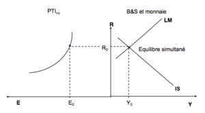
The IS-LM model does not make this assumption and gives us the simultaneous equilibrium conditions in the goods market (IS) and in the money market (LM) defined in the space { $Y$ ; $R$ }.

As we shall see, the conclusions reached in terms of the consequences for the macroeconomic balance following either a monetary or a fiscal shock are qualitatively identical to those obtained in the DD-AA model. The main advantage of the DD-AA model compared to the IS-LM model extended to the open economy is that it is better suited to analysing the long-term effects since the IS-LM model is a model based on the assumption of fixed prices.

The asset market: the AA curve[modifier | modifier le wikicode]

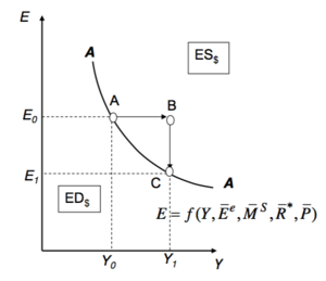
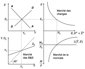
Definition: The AA curve is the set of pairs ( $Y$ , $E$ ) that simultaneously ensure equilibrium on the foreign exchange market ( $PTI_{nc}$ satisfied) and on the money market.

Derivation of the AA curve

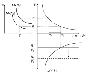
1) Graphic derivation :

Principle: we start from a situation of equilibrium ( $1-1'$ ), we consider a ↑ of $Y$ and we report the equilibrium combinations, ( $Y_{0}$ , $E_{0}$ ), ( $Y_{1}$ , $E_{1}$ ), in the diagram on the left.
Intuition: $Y$ ↑→ $L$ ↑ → $R$ ↑; to bring the asset market back to equilibrium this year ↑ of $R$ must be offset by currency appreciation ( $E$ ↓)

==> AA has a negative slope.

2) Synthetic Derivative :

point $A$ : simultaneous equilibrium in the asset and currency market $E$
point $B$ : $Y$ (income) ↑ => Currency ED => R↑ => ES currencies => $E$ ↓
point $C$ : nouvel équilibre simultané => AA a une pente négative.

All points above (below) AA correspond to a currency ES (ED).

Displacement of the AA curve[modifier | modifier le wikicode]

Example[modifier | modifier le wikicode]

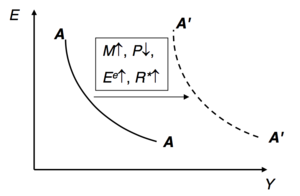
increase of $M$

Reasoning at constant $Y$ ( $R$ ↓) => moving AA upwards

NB: One could also have reasoned at constant $E$ ( $E={\bar {E}}_{0}$ ⟺ $R={\bar {R}}_{0}$ ); dn this case, to reabsorb the money ES at constant $R$ , it is necessary that $Y$ ↗ = moving AA to the right.

Generalisation[modifier | modifier le wikicode]

Any factor causing a currency ED ( $M$ ↗, $P$ ↓, $E^{e}$ ↗, $R*$ ↗) causes AA to move to the right.

Conversely: Any factor causing a currency ES ( $M$ ↓, $P$ ↗, $E^{e}$ ↓, $R^{*}$ ↓) moves the AA curve to the left.

The goods market: the DD curve[modifier | modifier le wikicode]

Global demand: assumptions[modifier | modifier le wikicode]

$C$ = private consumption

is positively dependent on disposable income ( $Y_{d}\equiv Y-T$ ) ⇒ $C=C(Y_{d})$ , where $0<{\frac {\partial C}{\partial Y}}\equiv c<1$ (marginal propensity to consume)

$I$ = business investment

assumed constant (exogenous) ⇒ $I={\bar {I}}$

$G$ = state spending and $T$ = taxes.

assumed constant (exogenous) ⇒ $G={\bar {G}}$ and $T={\bar {T}}$

$CA$ = "current account", to transfers on loan, i.e. $CA=EXP-IMP+SBRF$ , where we assume $SBRF$ constant and equal to $0$ ⇒ the current balance coincides with the trade balance.

The higher the $Y$ is, the higher the $IMP$ is, which deteriorates $CA$ (one neglects $Y^{*}$ which influences $EXP$ ). The higher the $q$ is, the higher the relative price of foreign products, which improves $CA$ (under a particular condition supposedly satisfied) ⇒ $CA=CA(Y,q)$ , où ${\frac {\partial CA}{\partial Y}}<0$ and ${\frac {\partial CA}{\partial q}}>0$

CA: Marshall-Lerner's Condition[modifier | modifier le wikicode]

Condition for ${\frac {\partial CA}{\partial q}}>0$

Link CA - q: if $q$ ↗, what's going on?

quantity effect: if $q$ ↗ => $EXP$ ↗, $IMP$ ↘ => goes well in the direction of a ↗ of CA.
price effect: if $q$ ↗ => the value of imports is increasing (their relative price ↗) => tendency towards ↘ of CA.

=> Ambiguous a priori effect.

It can be shown that, following a real depreciation, the current account balance will improve if the following condition is satisfied :

\eta +|\eta ^{*}|>1

where $\eta$ and $\eta ^{*}$ indicate the elasticity of demand for exports and the elasticity of demand for imports of the domestic country, respectively. This condition is known as the Marshall-Lerner (M-L) condition. Unless otherwise indicated, it is assumed that this condition is satisfied and that, therefore, a real depreciation of the domestic economy is not necessary. ( $q$ ↑) causes an improvement in CA.

Condition of M-L: J-curve[modifier | modifier le wikicode]

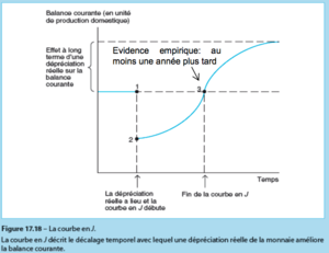
Empirical evidence shows that the initial effect of a depreciation on the current account is negative = the depreciation initially causes a deficit.

Explanation: the quantities imported and exported by enterprises and households are fixed in contracts, which will only be gradually renegotiated = initially only the price effect is active (the value of IMP ↑ while the value of EXP does not change), the quantity effect only appears later = initial negative effect on the balance of turnover.

J-curve :

The price effect of a devaluation is immediate (more expensive imports, with unchanged import and export quantities).
The quantity effects (sum of the elasticities) are slower on the J curve of CA versus time.

M-L condition: empirical evidence[modifier | modifier le wikicode]

"Short term" = < 6 months
"Medium term" = < 12 months
"Long term" = > 1 year

Our hyp. for the rest:

{\frac {\partial CA}{\partial q}}>0

Source: Krugman-Obstfeld

Balance in the G&S market[modifier | modifier le wikicode]

Balance on the goods and services market: Supply = Aggregate demand, i.e. :

Y=D_{g}(Y,E)=C(Y_{+d}+I+G+CA(Y_{-},q_{+})

Definition: the DD curve is the set of couples ( $Y$ , $E$ ) which ensure the equilibrium on the B&S market.

Assumptions:

${\frac {\partial C}{\partial Y_{d}}}\equiv c$ , marginal propensity to consume, $0<c<1$
${\frac {\partial CA}{\partial Y}}\equiv -mi$ , marginal propensity to import, $0<mi<c$
${\frac {\partial CA}{\partial _{q}}}>0$ , Marshall-Lerner's condition is met.

=> $D_{g}(Y_{+},q_{+}$ et $0<{\frac {\partial D_{g}}{\partial Y}}=c-mi<1$ = the overall demand is positively dependent on $Y$ (but the induced increase of $D_{g}$ is smaller than the increase of $Y$ ) and $q$ .

Equilibrium (short-term = fixed prices and variable $Y$ ) : $YD_{g}(Y,{\bar {E}},...)$

The G&S market: the DD curve[modifier | modifier le wikicode]

Derivation of the DD curve

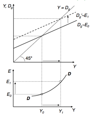
1) Graphic derivation:

Principe: we start from a situation of equilibrium, we consider a ↗ of $E$ (=> $q$ ↗ => by M-L, $CA$ ↗ => $D_{g}$ moves up and $Y$ ↗ to bring the goods market back into equilibrium) and the equilibrium combinations, ( $Y_{0},E_{0}$ ),( $Y_{1},E_{1}$ ), are plotted in the bottom diagram.

=> DD has a positive slope.

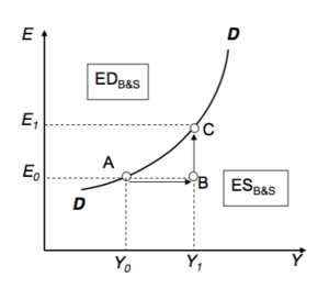
2) Synthetic derivative:

point $A$ : initial equilibrium
point $B$ : $Y$ (production)↗ => ES of G&S => E must ↗ (=> CA↗) to redress the balance
point $C$ : new balance

=> DD has a positive slope.

=> All points below (above) DD correspond to a G&S ES (ED).

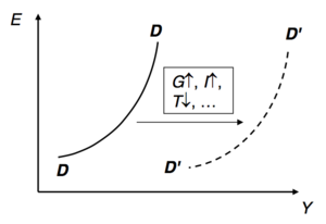
Displacement of the DD curve[modifier | modifier le wikicode]

Example: increase in G[modifier | modifier le wikicode]

By reasoning at constant $E$ ( $Y$ ↑) => dDD shift to the right

NB: one could also have reasoned at constant $Y$ -> $G$ ↑ -> $D_{g}$ ↑ => to restore balance by playing $E$ you need $E$ ↘ (⟺ $CA$ ↘)

=> moving DD down.

Generalisation[modifier | modifier le wikicode]

Any factor causing a G&S ED ( $G$ ↑, $T$ ↘, $P$ ↘, $P^{*}$ ↑, $c$ ↑, $mi$ ↘) causes DD to move to the right.

Conversely: Any factor causing a G&S ES ( $G$ ↘, $T$ ↑ , $P$ ↑ , $P^{*}$ ↘, $c$ ↘, $mi$ ↑ ) moves the DD curve to the left.

Long-term balance[modifier | modifier le wikicode]

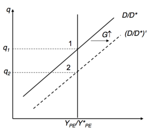
Alternative interpretation of [3] : $Y_{PE}=C(Y_{+PE}+I+G+CA(Y_{-PE},q_{+})$ [3’]

The condition [3'] determines the long term equilibrium level of $Y$ has been replaced by its full employment level ( $Y_{PE}$ ) => the condition [3'] determines the long term equilibrium level of $q$ (see chapter 13) :

Example : $G$ ↑ => ${\frac {D^{*}}{D}}$ ↑ => $q$ ↘

Reminder: it is this value of $q$ which

is involved in the expectations of $E$ :

E^{e}=(q)^{e}){\frac {P}{P^{*}}}

NB: the relative demand function for domestic products becomes decreasing if it is defined as ${\frac {1}{q}}$ or as ${\frac {D^{*}}{D}}$ .

The complete model[modifier | modifier le wikicode]

Equilibrium[modifier | modifier le wikicode]

The equilibrium values of $E$ , $Y$ and $R$ are those that simultaneously satisfy the equilibrium on the asset market (AA curve) and on the G&S market (DD curve).

Adjustment is faster in the asset market. E.g. point $1$ : $ES_{\$}$ and $ED_{B+S}$ => it is the foreign exchange market that adjusts the fastest ( $E$ ↘) => point $2$ : equilibrium restored in the asset market but $EDB_{B+S}$ remains => $Y$ ↗ gradually, but=> $L$ ↗ => $R$ ↗ => $E$ ↘ = we move along AA towards the simultaneous equilibrium of the three markets at the point $3$ .

Full Diagram[modifier | modifier le wikicode]

Determination of $Y$ , $E$ , $R$ (endogenous variables): the above DD-AA diagram is a kind of "reduced form model" of a "structural model".

Note: $Y_{0}\leq Y_{PE}$

Anticipated exchange rate ( $E^{e}$ )[modifier | modifier le wikicode]

In the full model, expectations of $E$ ( $E^{e}$ ) are determined by the following expression :

In the following chapters, we will use the full model to analyze monetary and fiscal policies under floating and fixed exchange rate regimes.

The IS-LM model in an open economy[modifier | modifier le wikicode]

IS-LM model[modifier | modifier le wikicode]

Curve IS (balance in the G&S market): $Y=D_{g}=C(Y-T,R-\pi ^{e})+I(R-\pi ^{e})+G+CA({\frac {EP^{*}}{P}},Y-T,R-\pi ^{e},Y^{*}-T^{*})$ , avec $G$ , $T$ , $Y^{*}$ et $T^{*}$ fixes

Curve LM (money market balance) : ${\frac {M}{P}}=L(R,Y)$

The $PTI_{nc}$ is checked in balance: $R=R^{*}+{\frac {E^{e}-E}{E}}$ → $E={\frac {E^{e}}{(1+R-R^{*}}}$

Our model therefore consists of three relationships =

$IS:Y=D_{g}({\frac {EP^{*}}{P}},Y-T,Y^{*}-T^{*},R-\pi ^{e},G)$ =>(negative slope in the space { $Y$ ; $R$ }, because the higher the income level, the lower the interest rate level has to be to find a balance between demand and supply of G&S)
$LM:{\frac {M}{P}}=L(R,Y)$ => (positive slope in the space { $Y$ ; $R$ } because the greater the $Y$ , the greater the interest rate must be to ensure the balance between real cash demand and real money supply).
$PTI_{nc}:R=R^{*}+{\frac {E^{e}-E}{E}}$ => (inverse relation between $R$ and $E$ which will allow us to see the impact of a monetary or fiscal policy on the exchange rate)

Displacement of the curves[modifier | modifier le wikicode]

Curve IS : any exogenous factor that increases aggregate demand causes the IS curve to shift to the right (at interest rate parity, $Y$ increases).
Curve LM : Any increase in the supply of money or reduction in demand (moving the money demand curve to the left) causes the LM curve to move to the right (the equilibrium interest rate falls for every $Y$ ).
$PTI_{nc}$ : see chapter 11.

Equilibrium[modifier | modifier le wikicode]

Summary[modifier | modifier le wikicode]

Model DD-AA[modifier | modifier le wikicode]

Curve AA :

combinations ( $E$ , $Y$ ) ensuring equilibrium in the asset market.
negative slope because if $Y$ ↗ => Money market EDs => $R$ ↗ => ES of currency => appreciation of the national currency = $E$ ↘.
Any factor leading to a currency ED moves AA to the right.

DD curve :

combinations ( $E$ , $Y$ ) ensuring equilibrium in the goods and services market.
positive slope because if $Y$ ↗ => ES on the G&S market actual depreciation required to restore equilibrium ⇔ $E$ must ↗.
Any factor leading to a B&S ED moves DD to the right.

Model IS-LM[modifier | modifier le wikicode]

IS curve :

combinations ( $Y$ , $R$ ) ensuring equilibrium in the goods and services market.
negative slope because if $Y$ ↗ => ES in the G&S market => ↘ $R$ to restore the balance.
Any factor leading to a B&S ED moves IS to the right.

LM curve :

combinations ( $Y$ , $R$ ) ensuring equilibrium in the money market.
positive slope because if $Y$ ↗ => ED in the G&S market => ↗ $R$ to restore the balance.
any factor leading to a currency ES moves LM to the right

Annexes[modifier | modifier le wikicode]

References[modifier | modifier le wikicode]

[1] Page personnelle de Federica Sbergami sur le site de l'Université de Genève

[2] Page personnelle de Federica Sbergami sur le site de l'Université de Neuchâtel

[3] Page personnelle de Federica Sbergami sur Research Gate

[4] Céline Carrère - Faculté d'économie et de management - UNIGE

[5] Céline Carrère - Google Scholar Citations

[6] Director Céline Carrère - Rectorat - UNIGE

[7] Céline Carrère | Sciences Po - Le Laboratoire Interdisciplinaire d'Evaluation des Politiques Publiques (LIEPP)

[8] Céline Carrere - EconPapers

[9] Céline Carrère's research works - ResearchGate

[1]

[2]

[3]

[4]

[5]

[6]

[7]

[8]

[9]

Introduction[modifier | modifier le wikicode]

DD-AA approach[modifier | modifier le wikicode]

IS-LM approach[modifier | modifier le wikicode]

The asset market: the AA curve[modifier | modifier le wikicode]

The asset market: the AA curve[modifier | modifier le wikicode]

Displacement of the AA curve[modifier | modifier le wikicode]

Example[modifier | modifier le wikicode]

Generalisation[modifier | modifier le wikicode]

The goods market: the DD curve[modifier | modifier le wikicode]

Global demand: assumptions[modifier | modifier le wikicode]

CA: Marshall-Lerner's Condition[modifier | modifier le wikicode]

Condition of M-L: J-curve[modifier | modifier le wikicode]

M-L condition: empirical evidence[modifier | modifier le wikicode]

Balance in the G&S market[modifier | modifier le wikicode]

The G&S market: the DD curve[modifier | modifier le wikicode]

Displacement of the DD curve[modifier | modifier le wikicode]

Example: increase in G[modifier | modifier le wikicode]

Generalisation[modifier | modifier le wikicode]

Long-term balance[modifier | modifier le wikicode]

The complete model[modifier | modifier le wikicode]

Equilibrium[modifier | modifier le wikicode]

Full Diagram[modifier | modifier le wikicode]

Anticipated exchange rate ( E e {\displaystyle E^{e}} )[modifier | modifier le wikicode]

The IS-LM model in an open economy[modifier | modifier le wikicode]

IS-LM model[modifier | modifier le wikicode]

Displacement of the curves[modifier | modifier le wikicode]

Equilibrium[modifier | modifier le wikicode]

Summary[modifier | modifier le wikicode]

Model DD-AA[modifier | modifier le wikicode]

Model IS-LM[modifier | modifier le wikicode]

Annexes[modifier | modifier le wikicode]

References[modifier | modifier le wikicode]

Anticipated exchange rate ( $E^{e}$ )[modifier | modifier le wikicode]